Chapter 34 Clustering

5 classes of clustering methods:
1. Partitioning methods - split into k-groups (k-means, k-dedoids (PAM), CLARA)
2. Hierarchical clustering
3. Fuzzy clustering
4. Density-based clustering
5. Model-based clustering

Clustering methods

• Representative-based
  • Each cluster has a representative point
  • May exist in the data or not. Also called centroid, center or prototype
  • Algorithms (K-means, Fuzzy C-Means, K-medoids or PAM, Expectation maximization)

Classification

• Connectivity-based
  • Create clusters based on their distance (closest points, farthest points, ect)
    
  • Hierarchical clustering
  • agglomerative (bottom-up)
  • divisive (top-down)
  • Algorithms (Ward, SLINK, CLINK, etc)
• Density-based
  • Cluster: area of higher density in the data
    
  • Data points can be categorized as core, border, noise
  • Algorithms (DBSCAN, OPTICS, Mean-shift)

Evaluation of clustering algorithms

• Types of validataion methods:
  • Internal: A quality metric computed on the data that was clustered (e.g., cluster compactness and separation)
    
  • External: Clustering is compared to “ground truth” classification.
    
  • Manual: Validated by a human expert.
    
  • Indirect: Evaluating its utility in the intended application.

34.1 Finding distances using factoextra

#Distances:
stats::dist()
factoextra::get_dist()   # compute a distance matrix between the rows of a data matrix
factoextra::fviz_dist()  # visualize distance matrix
cluster::daisy()         # handle both numeric and not numeric (nominal, ordinal,...) data types

34.2 Example of choosing clustering model

library(cluster)
library(factoextra)

d <- factoextra::get_dist(USArrests, stand = TRUE, method = 'pearson')
factoextra::fviz_dist(d, gradient = list(low='blue', mid='white', high='red'))

#####
library(tidyverse)
library(cluster)
library(factoextra)

data <- USArrests %>% na.omit() %>% scale()
data
factoextra::fviz_nbclust(data, kmeans, method = 'gap_stat')


km.res <- kmeans(data, 3, nstart = 25)
factoextra::fviz_cluster(km.res, data = data,
                         ellipse.type = 'convex',
                         palette = 'jco',
                         repel = TRUE,
                         ggtheme = theme_minimal())

# PAM clustering
pam.res <- cluster::pam(data, 4)
factoextra::fviz_cluster(pam.res)

# CLARA clustering
clara.res <- clara(df, 2, samples = 50, pamLike = TRUE)
clara.res

dd <- cbind(df, cluster = clara.res$cluster)

# Medoids
clara.res$medoids

# Clustering
head(clara.res$clustering,10)

34.3 K-means clustering

K-means assumptions

• Variables are all continuous
  
• Variables have a symmetric distribution (i.e., not skewed)
  
• Variables have similar means
  
• Variables have similar variance
  These assumptions come from the Euclidean distance
  Learned clusters will have a hyperspherical shape.

For variables taking only positive values -> apply logarithmic transformation
For variable swith negative values -> add a constant / calculate cubic root / Box-Cox transform

If variables have different ranges of numbers -> normalization is required

scale() base R function will standardize the data.

• K - number of clusters in K-means clustering.

• Optimal K produces compact, well-separated clusters.

• Compactness: Within-Cluster Sum of Squares (WSS).

  • minimize WSS: compact clusters!

• Separation: Between-Cluster Sum of Squares (BSS).
  maximize BSS: well-separated clusters!

• Problem: WSS decreases as K increases.

The elbow method
* Compute WSS, BSS, TSS = WSS + BSS * Select smallest k such that WSS / TSS < 0.2

kmeans() function in the stats package

34.4 k-Means

library(datasets)
head(iris)

##   Sepal.Length Sepal.Width Petal.Length Petal.Width Species id
## 1          5.1         3.5          1.4         0.2  setosa  1
## 2          4.9         3.0          1.4         0.2  setosa  2
## 3          4.7         3.2          1.3         0.2  setosa  3
## 4          4.6         3.1          1.5         0.2  setosa  4
## 5          5.0         3.6          1.4         0.2  setosa  5
## 6          5.4         3.9          1.7         0.4  setosa  6

# Plot Petal.Length ~ Petal.Width data
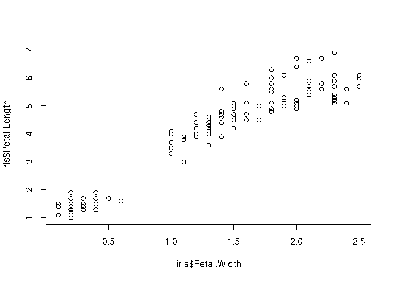
plot(iris$Petal.Length ~ iris$Petal.Width)

set.seed(20)

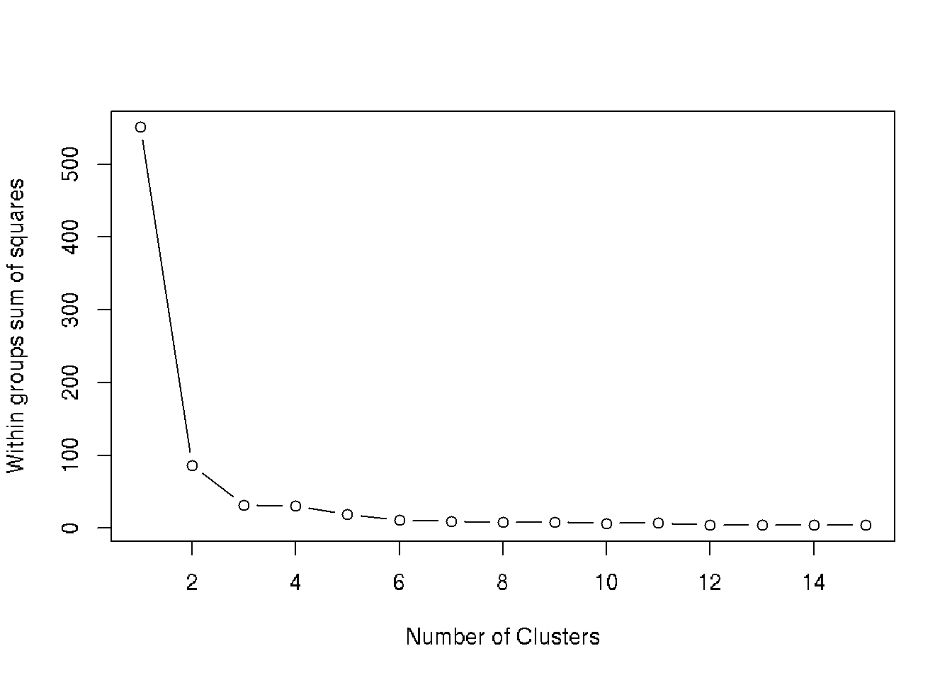
# Find number of clusters using wss
wss <- (nrow(iris[, 3:4])-1)*sum(apply(iris[, 3:4],2,var))
for (i in 2:15) wss[i] <- sum(kmeans(iris[, 3:4], i)$withinss)
plot(1:15, wss, type="b", xlab="Number of Clusters", ylab="Within groups sum of squares")

#More than 3 clusters give no obvious advantages

# Make k-means with 3 clasters
ncl <- 3
irisCluster <- kmeans(iris[, 3:4], ncl, nstart = 20)
irisCluster

## K-means clustering with 3 clusters of sizes 48, 50, 52
## 
## Cluster means:
##   Petal.Length Petal.Width
## 1     5.595833    2.037500
## 2     1.462000    0.246000
## 3     4.269231    1.342308
## 
## Clustering vector:
##   [1] 2 2 2 2 2 2 2 2 2 2 2 2 2 2 2 2 2 2 2 2 2 2 2 2 2 2 2 2 2 2 2 2 2 2 2 2 2 2 2 2 2 2 2 2
##  [45] 2 2 2 2 2 2 3 3 3 3 3 3 3 3 3 3 3 3 3 3 3 3 3 3 3 3 3 3 3 3 3 3 3 1 3 3 3 3 3 1 3 3 3 3
##  [89] 3 3 3 3 3 3 3 3 3 3 3 3 1 1 1 1 1 1 3 1 1 1 1 1 1 1 1 1 1 1 1 3 1 1 1 1 1 1 3 1 1 1 1 1
## [133] 1 1 1 1 1 1 3 1 1 1 1 1 1 1 1 1 1 1
## 
## Within cluster sum of squares by cluster:
## [1] 16.29167  2.02200 13.05769
##  (between_SS / total_SS =  94.3 %)
## 
## Available components:
## 
## [1] "cluster"      "centers"      "totss"        "withinss"     "tot.withinss" "betweenss"   
## [7] "size"         "iter"         "ifault"

# Compair result of clustering with real data (3 species of iris are in analysis)
table(irisCluster$cluster, iris$Species)

##    
##     setosa versicolor virginica
##   1      0          2        46
##   2     50          0         0
##   3      0         48         4

# Plot data
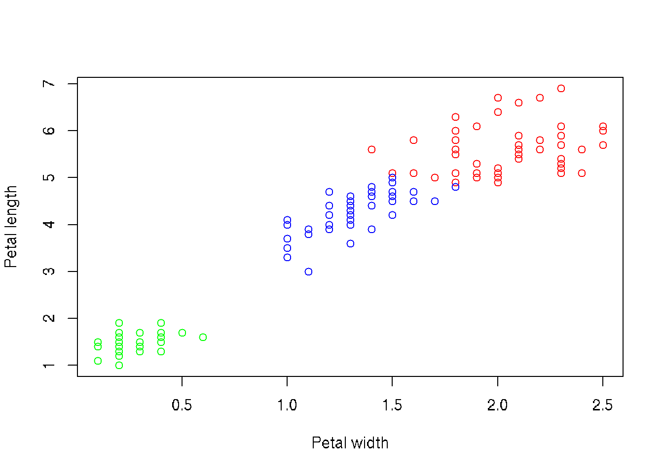
clusters <- split.data.frame(iris, irisCluster$cluster)
xlim <- c(min(iris$Petal.Width), max(iris$Petal.Width))
ylim <- c(min(iris$Petal.Length), max(iris$Petal.Length))
col <- c('red', 'green', 'blue')
plot(0, xlab='Petal width', ylab='Petal length', xlim=xlim, ylim=ylim)
for ( i in 1:ncl ) {
points(clusters[[i]]$Petal.Length ~ clusters[[i]]$Petal.Width, col=col[i], xlim=xlim, ylim=ylim)
}

34.5 Hierarchical clustering

bv <- read.table("./DATA/beverage.csv", header=T, sep=";")  
head(bv)  
# no needs to normalize because all data is binary (0,1)

# Hierarchical clustering
# dist - calculate distances
# hclust - hierarchical clustering

clust.bv <- hclust(dist(bv[,2:9]), "ward.D")
clust.bv

# Plot clusters
plot(clust.bv)
plot(clust.bv, hang = -1)
rect.hclust(clust.bv, k=3, border="red") 

# Group data by clusters
groups <- cutree(clust.bv, k=3)
groups

# Percentage in broups by drinking different beverages
colMeans(bv[groups==1, 2:9])*100
colMeans(bv[groups==2, 2:9])*100
colMeans(bv[groups==3, 2:9])*100

# Interpretation
# 1. People who does not have specific preference
# 2. People who prefers cola and pepsi
# 3. Not clear (others)

# atributes of cluster analysis
names(clust.bv)

# chronic of combining
clust.bv$merge
clust.bv[1]

clust.bv$height
clust.bv$order
clust.bv$labels
clust.bv$method
clust.bv$call
clust.bv$dist.method

# Detect the best choice for number of cluster by elbow-plot
plot(1:33, clust.bv$height, type="l")

### Task. Analyse data and find groups of people
# Scores (0,10) of 10 tests for candidates to get a job.
# 1. Memorizing numbers
# 2. Math task
# 3. Solving tasks in dialoge
# 4. Algorithms
# 5. Self confidence
# 6. Work in group
# 7. Find solution
# 8. Collaboration
# 9. Acceptance by others

setwd("~/DataAnalysis")
job <- read.table("DATA/assess.dat", header=T, sep="\t")
job

# Clustering
clust.job <- hclust(dist(job[,3:ncol(job)]), "ward.D")
# no needs to normalize, because all numbers have the same min, max
plot(clust.job)  # visual number of clusters is 4

# Group data by clusters
groups <- cutree(clust.job, k=4)
groups
colMeans(job[groups==1, 3:12])*100

### Find clusters using k-means method

setwd("~/DataAnalysis")
bv <- read.table("DATA/beverage.csv", header=T, sep=";")
bv
dim(bv)
names(bv)

# k-means clustering, with initial 3 clusters
# nstart = x - run x times with different initial clusters
summ.1 = kmeans(bv[,2:9], 3, iter.max = 100)
names(summ.1)

# Objects by clusters
summ.1$cluster

# Centers of clusters
summ.1$centers
# 2 digits after point
options(digits=2)

t(summ.1$centers)
options(digits=7)

# Square summs
summ.1$withinss

# Summ of elements of vector
summ.1$tot.withinss

# sum(33*(apply(bv[,2:9], 2, sd))^2)
summ.1$totss
summ.1$tot.betweenss

# Size of clusters
summ.1$size

# Elbow plot to detect optimal number of clusters
wss <- (nrow(bv[,2:9])-1)*sum(apply(bv[,2:9],2,var))
for (i in 2:15) { wss[i] <- kmeans(bv[,2:9],
                centers=i)$tot.withinss }
plot(1:15, wss, type="b", xlab="Number of Clusters",
     ylab="Within groups sum of squares")

# We can see that diagram is rough. This is because clusters are not allways optimal
# To improve situation, we have to run many initiall start coordinates and choose the best
# option (add nstart=500):
wss <- (nrow(bv[,2:9])-1)*sum(apply(bv[,2:9],2,var))
for (i in 2:15) { wss[i] <- kmeans(bv[,2:9],
                                   centers=i, nstart=500)$tot.withinss }
plot(1:15, wss, type="b", xlab="Number of Clusters",
     ylab="Within groups sum of squares")
# Warnings means that iterations were not finished for some cases.

# Let's compair results for 3 and 4 clusters
summ.1 = kmeans(bv[,2:9], 3, iter.max=100)
summ.2 = kmeans(bv[,2:9], 4, iter.max=100)

# Compair clusters. How many elements in each cluster
# We can see how elements move if we take more clusters
table(summ.1$cluster, summ.2$cluster)

# Multidimentional scaling
# Project multidimentional data to 2d
bv.dist <- dist(bv[,2:9])
bv.mds <- cmdscale(bv.dist)
plot(bv.mds, col = summ.1$cluster, xlab="Index", ylab="")

# Detect optimal number of clusters
install.packages("NbClust")
library("NbClust")
Best <- NbClust(bv[,2:9],              # data 
                distance="euclidean",  # distance method
                min.nc=2,              # min number of clusters
                max.nc=8,             # max number of clusters
                method="ward.D",       # ward methodes 
                index = "alllong" )    # choose indices

34.6 KNN

# K-Nearest Neighbors or KNN is a clustering algorithm
# k is known number of clusters (usually sqrt(N), between 3-10, but may be different)
# samples must be normalized x = (x - min(x))/(max(x)-min(x))

head(iris)
summary(iris)   # detailed view of the data set
str(iris)   # view data types, sample values, categorical values, etc
plot(iris)

#normalization function

min_max_normalizer <- function(x)
{
    num <- x - min(x) 
    denom <- max(x) - min(x)
    return (num/denom)
}

#normalizing iris data set
normalized_iris <- as.data.frame(lapply(iris[1:4], min_max_normalizer))

#viewing normalized data
summary(normalized_iris)

#checking the data constituency
table(iris$Species)

#set seed for randomization
set.seed(1234)

# setting the training-test split to 67% and 33% respectively
random_samples <- sample(2, nrow(iris), replace=TRUE, prob=c(0.67, 0.33))

# training data set
iris.training <- iris[
    random_samples ==1, 1:4] 

#training labels
iris.trainLabels <- iris[
    random_samples ==1, 5]


# test data set
iris.test <- iris[
    random_samples ==2, 1:4]

#testing labels
iris.testLabels <- iris[
    random_samples ==2, 5]

#setting library
library(class)

#executing knn for k=3
iris_model <- knn(train = iris.training, test = iris.test, cl = iris.trainLabels, k=3)

#summary of the model learnt
iris_model