Chapter 8 Data normalization

Data normalization (feature scaling) is not always needed for e.g. decision-tree-based models.

Data normalization is beneficial for:

• Support Vector Machines, K-narest neighbors, Logistic Regression
• Neural networks
  
• Clustering algorithms (K-means, K-medoids, DBSCAN, etc.)
  
• Feature extraction (Principal Component Analysis, Linear Discriminant Analysis, etc)

Min-max scaling

• Maps a numerical value \(x\) to the [0,1] interval

\[x' = \frac{x - min}{max - min}\]

• Ensures that all features will share the exact same scale.
  
• Does not cope well with outliers.

Standardization (Z-score normalization)

• Maps a numerical value to \(x\) to a new distribution with mean \(\mu = 0\) and standard deviation \(\sigma = 1\)

\[x' = \frac{x - \mu}{\sigma}\]

• More robust to outliers then min-max normalization.
  
• Normalized data may be on different scales.

Example

library(dplyr)

# generate data with different ranges
df <- data.frame(
    a = sample(seq(0, 2, length.out=20)),
    b = sample(seq(100, 500, length.out=20)))
# view data
glimpse(df)

## Rows: 20
## Columns: 2
## $ a <dbl> 1.3684211, 1.1578947, 1.2631579, 2.0000000, 0.7368421, 1.5789474, 0.0000000, 1.05…
## $ b <dbl> 331.5789, 457.8947, 394.7368, 184.2105, 247.3684, 310.5263, 121.0526, 100.0000, 1…

# data ranges to see if normalization is needed
sapply(df, range)

##      a   b
## [1,] 0 100
## [2,] 2 500

# ranges are different => normalize
# Apply min-max and standardization
nrm <- df %>% 
    mutate(a_MinMax = (a - min(a)) / (max(a) - min(a)), 
           b_MinMax = (b - min(b)) / (max(b) - min(b)),
           a_ZScore = (a - mean(a)) / sd(a),
           b_ZScore = (b - mean(b)) / sd(b)
    )

# ranges for normalized data
sapply(nrm, range)

##      a   b a_MinMax b_MinMax  a_ZScore  b_ZScore
## [1,] 0 100        0        0 -1.605793 -1.605793
## [2,] 2 500        1        1  1.605793  1.605793

# plots
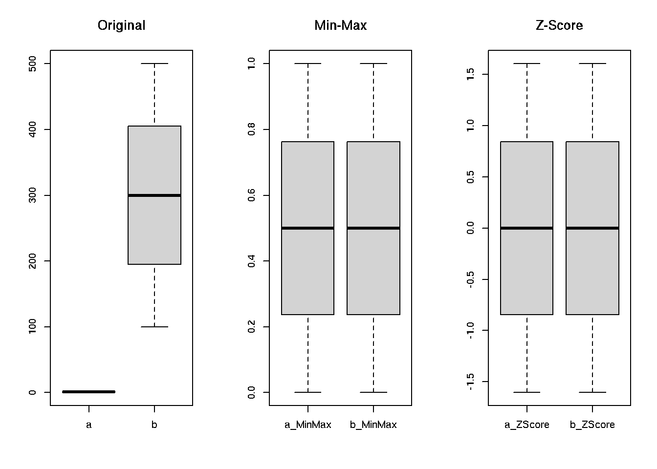
par(mfrow=c(1,3))
boxplot(nrm[, 1:2], main = 'Original')
boxplot(nrm[, 3:4], main = 'Min-Max')
boxplot(nrm[, 5:6], main = 'Z-Score')

8.1 Normality test

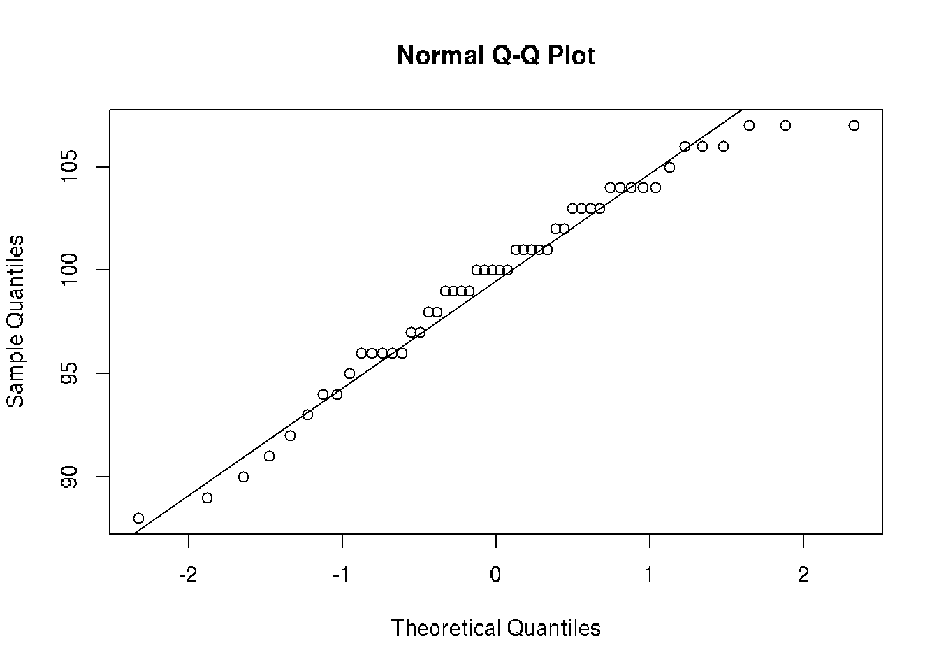
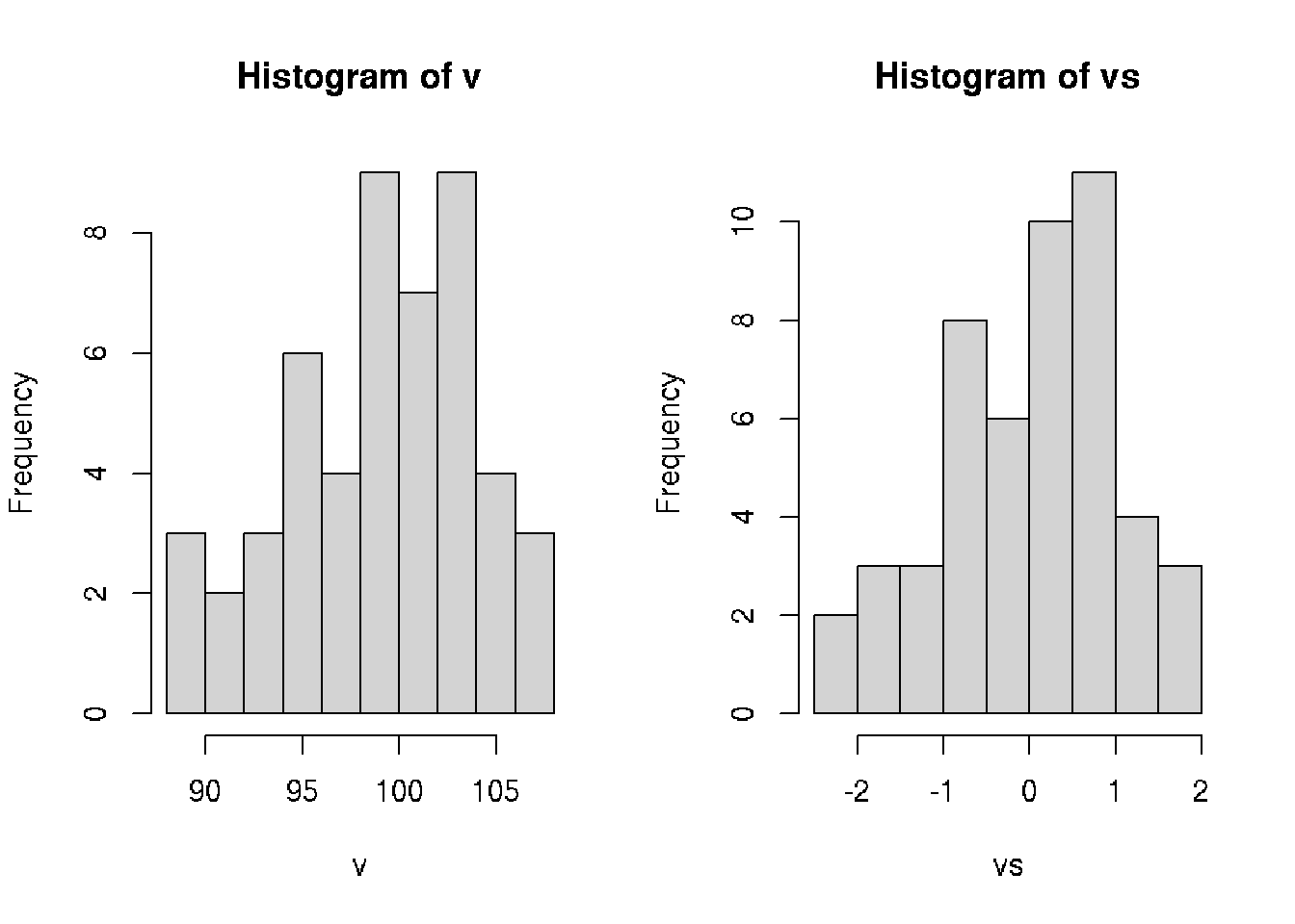
It is possible to use histogram to estimate normality of the distribution.

# QQ-plot - fit normal distibution
qqnorm(v); qqline(v)

var(v)     # variance: sd = sqrt(var)

## [1] 23.76367

sd(v)      # standard deviation

## [1] 4.8748

sd(v)/sqrt(length(v))  # standard error sd/sqrt(n)

## [1] 0.6894008

# Z-score (standartization)
# transform distribution to mean=0, variance=1
# z = (x - mean(n))/sd
vs <- scale(v)[,1]
vs

##  [1] -1.75186680  0.29949948  0.50463610 -2.16214006  0.91490936 -0.11077378 -0.72618366
##  [8]  0.70977273  1.53031924  0.09436285  0.50463610  0.29949948 -0.93132029  0.29949948
## [15] -0.72618366  1.12004599 -0.11077378 -0.72618366  0.29949948 -1.13645692 -0.72618366
## [22] -0.11077378 -1.13645692 -1.34159355  0.70977273  0.09436285  0.09436285  0.29949948
## [29]  1.53031924 -0.31591041  1.32518262 -0.52104703 -1.95700343  1.32518262  0.70977273
## [36] -0.11077378  0.91490936  0.91490936  0.91490936  1.32518262  0.70977273  0.09436285
## [43] -2.36727668  1.53031924 -0.31591041 -0.72618366 -1.54673017  0.91490936  0.09436285
## [50] -0.52104703

par(mfrow=c(1,2))
hist(v, breaks=10)
hist(vs, breaks=10)

8.2 Finding Confidence intervals

# sample of random integers
x <- round(rnorm(n=50, sd=5, mean=100))

# Confidence interval for normal distribution with p=0.95
m <- mean(x)
s <- sd(x)
n <- length(x)
error <- qnorm(0.95)*s/sqrt(n)
confidence <- c(m-error, m+error)
confidence

## [1]  99.16802 101.19198

# Confidence interval for t-distribution with p=0.95
a <- 5
s <- 2
n <- 20
error <- qt(0.975,df=n-1)*s/sqrt(n)
# confidence interval
c(left=a-error, right=a+error)

##     left    right 
## 4.063971 5.936029

Sources
Practicing Machine Learning Interview Questions in R on DataCamp